Quick Links
Picture this—you have a large workbook full of nicely formatted, filtered, and sorted tables. You might think that your work is done, but actually, Excel is sitting and waiting for you to do more with those tables, eager to help you make the most of the hard work you have done so far.
In this article, I’ll run through three of the functions or combinations of functions I use the most when I want to either extract or summarize information in my Excel tables.

VLOOKUP and HLOOKUP
VLOOKUPand HLOOKUP are both used to locate and retrieve a value from specific locations in a table.
VLOOKUP
Here, I have a list of exam grades and the scores required for each grade (let’s call this table 1). I also have a table containing students' scores (table 2 from this point). I want Excel to use the information in table 1 to complete the missing column in table 2.
I will use VLOOKUP, because I want Excel to look up the values in the first column of table 1 to return each student’s grade in table 2. The VLOOKUP function has the following syntax:

where
So, in my case, I’ll type this formula into cell F2 to work out Tom’s grade, before usingAutoFillto look up the other grades in the table:

I’ve used $ symbols to create anabsolute referencefor valuebabove, as I want Excel to continually use cells A1 to B9 to look up the values. I’ve also used “TRUE” for valued, as the score boundary table contains ranges, and not a grade assigned to individual scores.
HLOOKUP
Here, we have the same grade boundary information, but this time, it’s displayed horizontally. This means the data we want to fetch is in the second row of the boundary table.
So, I’ll type this formula into cell C5 to work out Tom’s grade, before usingAutoFillto look up the other grades in the table:

INDEX With MATCH
Another effective way to look up and retrieve values is throughINDEX and MATCH, especially when used together. INDEX finds and returns a value in a defined location, while MATCH finds and returns the location of a value. Together, they enable dynamic data retrieval.
Individual Syntaxes
Before we look at using these functions together, let’s briefly look at them individually.
The syntax for INDEX is

whereais the range of cells containing the data,bis the row number to evaluate, andcis the column number to evaluate.
On this basis,

would evaluate cells B2 to D8, and return the value in the fourth row and second column within that range.
For MATCH, we follow

wherexis the value we’re looking up,yis the range where the value is to be found, andz(optional) is the match type.
would tell me where the number 5 is located within the range B2 to B8, and the0tells Excel to perform an exact match.

Used Together
In this example, I want Excel to tell me the number of goals a specified player has scored in a given month. More specifically, I want to know how many goals player C has scored in the third month, but I’m going to create this formula so that I can change these criteria at any time.
To achieve this, I need Excel to determine where player C is in the table, and then tell me what value is in the third column of the data.
In cell G4, I’ll start with the INDEX function, as I want Excel to find and return a value from my raw data. Then, I’ll tell Excel where to look for that data.
The next part of the INDEX syntax is the row number, and this will vary depending on which player I state in cell G2. For example, if I want to look up player A, it’ll be the first row. To do this, I’ll initiate the MATCH function, as I want Excel to match the player I’ve typed into cell G2 with the corresponding cell in the player column (A2:A8), and work out which row number it’s on. I’ve also added a0at the end, as I want Excel to return an exact retrieval.

Now that I’ve told Excel the row number for the INDEX function, I need to finish with the column number. In my case, the column number represents the month number I’ve typed into cell G3.
When I press Enter, Excel correctly informs me that player C scored five goals in the third month.
Now, I can change any of the values in my lookup table to find any player’s total for any of the months.
COUNTIF and SUMIF
As you may gather from their names, these two functions count and sum values based on criteria you set. Anything not included within your criteria will not be added or counted, even if it’s within the range you specify.
COUNTIFcounts cells containing certain criteria. The syntax is
whereais the range you want to count, andbis the criteria for counting.
Similarly, if I wanted to include more than one criterion, I’d use COUNTIFS:
whereaandbare the first range-criteria pairing, andcanddare the second range-criteria pairing (you can have up to 127 pairings).
If any criteria are text or a logical or mathematical symbol, they must be enclosed in double-quotes.
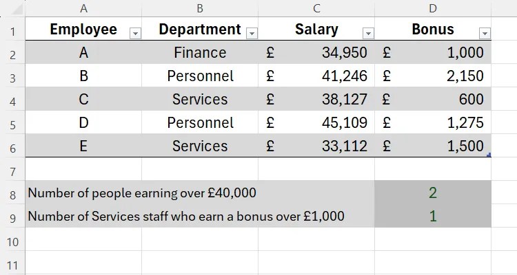
In my salary table below, I want to calculate the number of people earning over £40,000 and, separately, the number of service staff who earn a bonus of over £1,000.
To count the number of workers with a salary of over £40,000, I need to type this formula into cell D8:
whereC2:C6is the range where the salaries are located, and">40000"is the criterion.
To calculate the number of service personnel who earn bonuses of over £1,000, I would use COUNTIFS, as I have two criteria.
TheB2:B6,“Services"part is the first range-criterion pairing, andD2:D6,">1000"is the second.
Even though there are commas separating the thousands in my table above, I haven’t included these within the formula, as commas have a different function in this context.
SUMIF
SUMIFsums cells based on criteria you set. It works on a similar principle as COUNTIF, but with more arguments in the parentheses. The syntax is
whereais the range of cells you want to evaluate before making the sum,bis the criteria for that evaluation (this can be a value or a cell reference), andc(optional) is the cells to add if different toa.
This time, we have three things to work out: the sum of the salaries over £40,000, the total salary for the service department, and the sum of the bonuses for staff whose salary is over £35,000.
First, to work out the sum of the salaries over £40,000, I need to type the following formula into cell D8:
whereC2:C6references the salaries in the table, and”>40000"tells Excel to only sum the values over this amount.
Next, I want to find out the total salary for the services department. So, in cell C9, I’ll type
whereB2:B6references the department column,“Services"tells Excel that I’m looking specifically for employees in the services department, andC2:C6tells Excel to sum the salaries of these employees.
My last task is to find out how much employees earning over £35,000 have made in bonuses. In cell C10, I’ll input
whereC2:C6tells Excel to evaluate the salaries,">35000"is the criterion for those salaries, andD2:D6tells Excel to sum the bonuses of those individuals who fulfill the criterion.
Excel also has a SUMIFS function, which carries out the same process but for more than one criterion. It has a very different syntax to SUMIF:
whereais the range of cells to sum,bis the first range that is evaluated,cis the criterion forb, anddandeare the next range-criterion pairing (you can have up to 127 pairs).
Using the table above, let’s say I wanted to sum up the bonuses for personnel staff earning over £45,000. Here’s the formula I would type:
Once you’ve mastered the functions detailed above, trythe XLOOKUP function, which aims to address some of VLOOKUP’s shortcomings by looking up values to the left and right of the lookup value column without you having to rearrange your data.
